Visual comparison of Global Illumination Methods
Summary
I wanted to compare the different Global Illumination algorithms, for one of my lectures. I took a simple test scene, the Lexus CS 2054, by 3dregenerator, on TF3DM.
Importing it into the Mitsuba renderer was straightforward. I changed the following materials: "windows" and "windows_black" to a transparent dielectric, "chrom" to a conductor.
I then ran several illumination algorithms on the scene:
- Path Tracing,
- Bi-Directional Path-Tracing,
- Photon Mapping,
- Metropolis Light Transport,
- Manifold Exploration Metropolis Light Transport
- Progressive Photon Mapping
- Stochastic Progressive Photon Mapping
As much as possible, I tried to run with the default parameters. When it isn't the case, I'll mention it in the text.
All computation times and pictures correspond to Mitusba, version 0.5.0, running on a MacBook Air, with a 1.7 GHz Core i7 processor, and 8GB of RAM.
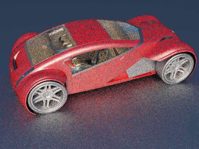
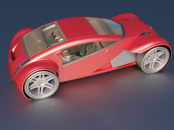
Path Tracing
A straightforward method. A single parameter, the number of samples per pixel

|

|

|

|
| 1 spp (0.7 s) | 32 spp (21 s) | 256 spp (3 mn) | 1024 spp (12.4 mn) |
This method converges nicely on the outside of the car, but has problems with the inside. Light paths contributing to illumination inside the car have to go through the windows, which prevents direct lighting.
One of the advantages is that the anti-aliasing on the edges of the car is really fantastic.
Using adaptive sampling rates (the adaptive integrator in Mitsuba) improves the quality:

|
| 256 to 8192 spp (53 mn) |
Bi-Directional Path-Tracing
Bi-Directional Path Tracing also takes a single parameter, the number of samples per pixel.
|

|

|

|
| 1 spp (2 s) | 32 spp (42 s) | 256 spp (5.4 mn) | 1024 spp (23 mn) |
It converges faster on the outside, even though it takes more time than Path-Tracing for the same number of samples. Inside, it reverts to path-tracing behavior.
Photon Mapping
Here, we have several parameters to adjust: number of global photons, number of caustic photons, number of samples per pixel, whether or not we use a Final Gather. For this integrator, I had to use the parameter autoCancelGathering=false.

|
|
|

|
| 10 K global photons 10 K caustic photons 32 spp, no FG, 19.5 mn |
10 K global photons 10 K caustic photons 32 spp, with FG (20.3 mn) |
100 K global photons 100 K caustic photons 32 spp, no FG (1.8 h) |
10 K global photons 10 K caustic photons 256 spp, no FG (1.3 h) |
The only parameter that appears to have an influence on image quality is the number of samples per pixel. The Final Gathering step has no visible influence, probably because this scene contains no diffuse surfaces.
Increasing the number of photons does not seem to influence the picture quality, even though it does change the computation time.
Using adaptive sampling rates (the adaptive integrator in Mitsuba) improves the quality, with a reasonnable impact on computation time:

|
| 100 K global photons, 100 K caustic photons 256 to 8192 spp (2.3 h) |
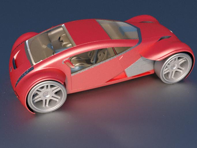
Metropolis Light Transport
Metropolis Light Transport takes a single parameter, the number of mutations or perturbations per pixel.

|
|
| 1024 mutations per pixel (11.8 mn) | 2048 mutations per pixel (23.2 mn) |
Hard-to-find caustics, such as those inside the car, but also next to the rightmost wheel, appear blotchy. The algorithm has trouble finding them, and when it does, it gives them too much importance.
Overall, a much better result than BDPT for the same computation time.
I'm a little unsatisfied by the aliasing on the edges of the gray stripe on the car door.
Manifold-Exploration Metropolis Light Transport
Again, a single parameter: the number of mutations per pixel.

|
|
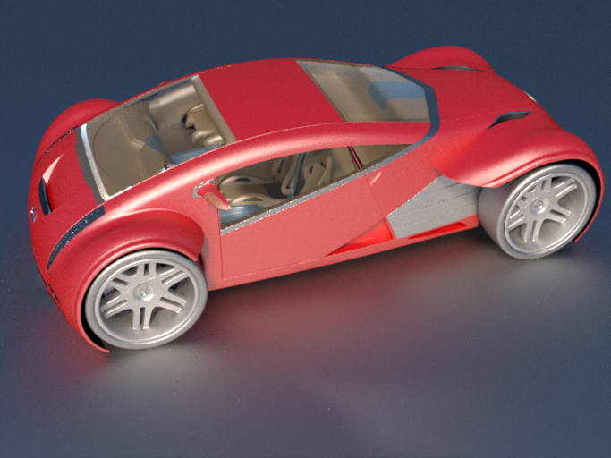
|
| 1024 mutations per pixel (17 mn) | 2048 mutations per pixel (27 mn) | 4096 mutations per pixel (54 mn) |
Very good quality for the computation time (compare to BDPT for 23 mn). On the other hand, it appears to have missed the two small caustics in on the floor caused by the logos on the wheel hubs. Almost all the other methods found them.
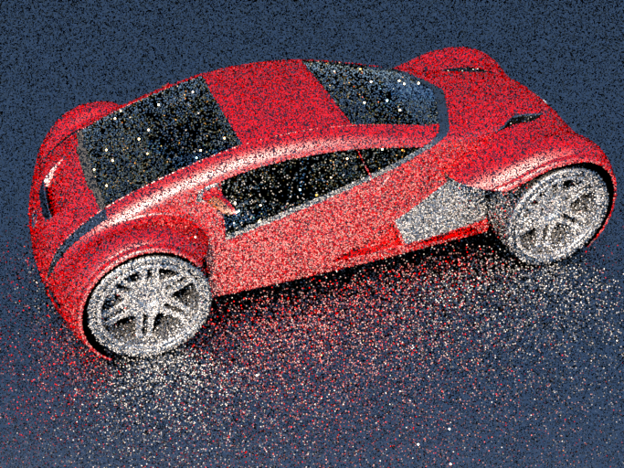
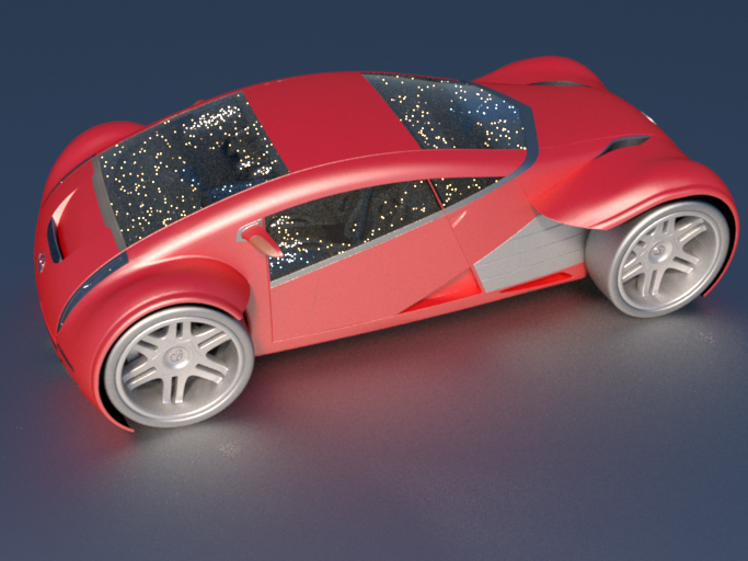
Progressive Photon Mapping
This method does not have parameters. Results only depend on computation time.
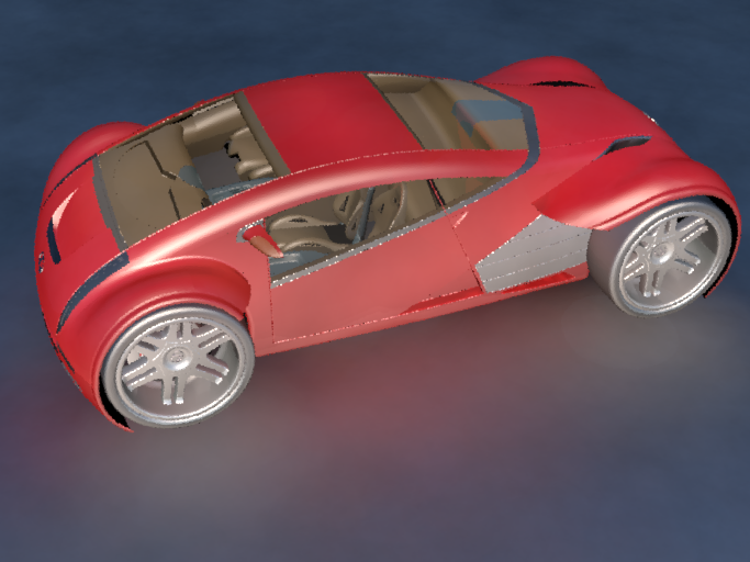
|

|

|
|
| 14 mn | 25 mn | 46 mn | 76 mn |

|

|
||
| 4 h | 6 h |
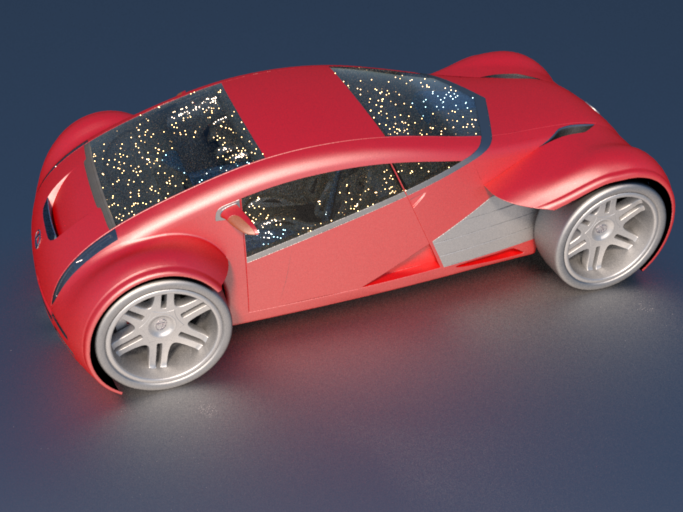
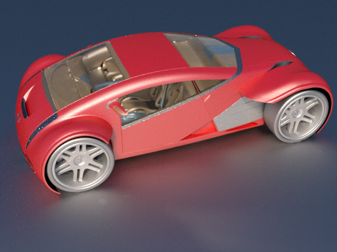
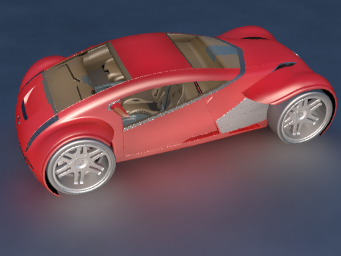
Stochastic Progressive Photon Mapping
Again, a method with no parameters. Results only depend on computation time.

|
|

|

|
| 12 mn | 23 mn | 85 mn | 2h 20mn |
|
|||
| 13 h |